
Meniscus Habitat Assessment
GSP 533 Spring 2016 Session C
John Bonifas
5/17/2016
Hedeoma diffusum (Flagstaff Pennyroyal) is a small perennial herb that grows in central Arizona, mainly in alpine areas surrounding Flagstaff between 4500 and 7000 feet in elevation. It prefers shallow soil in exposed limestone outcrops and cracks.
Hedeoma diffusum is currently threatened by development, heavy grazing, and ORV activities. The authorities have recommended that it be added to the Arizona Native Plant Law protected plants list, and it is about to receive an official status of Threatened by the U.S. Fish and Wildlife Service.
We performed the following tasks in this project:
We started by obtaining vector and raster data to be used for further editing and analysis. That included coordinate data from the BLM, and raster data in DRG format. Once we had the study area delineated in the GIS software, we created vector feature classes that define the roads, rivers, soil types, tree coverage, water tanks, power lines, and other vector entities that are located in the Meniscus study area.
After importing all completed GIS feature class layers into a geodatabase, we added the required raster data and perform various spatial analysis techniques to determine where potential meniscus habitat sites might be, that are an appropriate distance away from human activity. Finally, we created a spatial model that predicts soil depth for the Meniscus project area.
A comprehensive schema of all data used and manipulated in this project is in Appendix A.
The criteria we chose to determine ideal potential plant habitats are listed below:
Preparation for analysis began by creating a new geodatabase, and importing several features, including a table with vegetation type data, a feature class representing the tree canopy, and a feature class representing the roads crossing the study area.
Our first step was to determine areas of potential Meniscus habitat. We determined which roads crossed ponderosa pine stands in the study area by merging the tree canopy layer with the vegetation type table, selecting only the Ponderosa Pine forest type, then selecting by intersection. To determine which water tanks on private lands were within a 300' distance of a road in the study area, we did a select by proximity, then filtered by owner and by containment within private land.
We then imported a soil feature class and soil type attribute table, merged the two, filtered two soil types out, then performed an intersect overlay between the soil types feature and the canopy/vegetation feature. This produced a feature class that identified new potential plant habitat areas.
We then created a road buffer feature, and performed an intersect overaly to determine areas that were both private land and within the road buffer distance. Finally we performed an intersect overlay with the habitat areas feature and the human activity feature, to create a feature containing potential plant habitat areas away from human activity.
At this point, we had an analysis of all the above habitat criteria except one - sunny slopes. This required a 3-step separate digital terrain analysis process, described as follows. First, we downloaded the required USGS Digital Elevation Model blocks for the study area, and because we were using ArcGIS software for the analyses, we converted the DEMs to ESRI GRIDs. Some of the models were in STDS format, and 1 large model came from the National Elevation Dataset. These were also converted to ESRI GRIDs.
Once the 4 GRIDs were created, we used a python script and map algebra to perform a merge of the GRIDs. Because the rest of our data was projected into UTM zone 12, and the resultant GRID raster was not projected as GCS in NAD 1983, we used ArcCatalog to reproject it into UTM 12.

We were now prepared to perform the required digital terrain analyses. All analysis tools we used were located in the ArcGIS Spatial Analyst toolbox. Our main input data to the slope and solar aspect analyses, in addition to several others, was the DEM of the Meniscus study area.
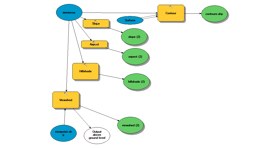
We used the contour tool to create a feature class containing the elevation contours for the study area. All other analysis outputs were rasters. We used the Aspect tool to create the solar aspect raster, and the Slope tool to create the slope raster.
The analysis used to define a watershed for the Meniscus study area was entirely automated using the ArcGIS Python facility. A workflow for the analysis is shown below.

Here, we used the Fill and Flow Direction Spatial Analyst tools to create intermediate input rasters that we fed into the Watershed tool, creating the shape of the watershed, shown below.

We now had all the data representing the criteria we listed above to begin building the soil depth prediction model; we just needed to do some preliminary preprocessing to the input rasters, so that they would be valid parameters to the model building tool. We also obtained a feature class containing the soil depth at some sample locations within the study area.
We used map algebra to modify certain rasters to filter out undesired data. To modify our solar aspect raster so that it only contained southern facing slopes, we filtered out slopes in the undesired direction. So that our input canopy raster contained only ponderosa pine stands, we filtered out non ponderosa pine stands. So that our soil types raster contained only eutroboraif soils, we filtered the rest out.
We then used the Extract Values To Points tool on the above rasters, and the soil depth samples, to convert them into their respective feature class equivalents. To create proximity data of each sample location to the nearest stream channel, we ran the sample points feature class and a feature class containing stream locations in the study area through the Spatial Analyst Near Tool.
So that all calculated data for the prediction model would be in the same feature class input file, we created fields for each criteria parameter in the sample points feature class, and copied all prepared data for all parameters to the model building tool into the sample points feature class input file.
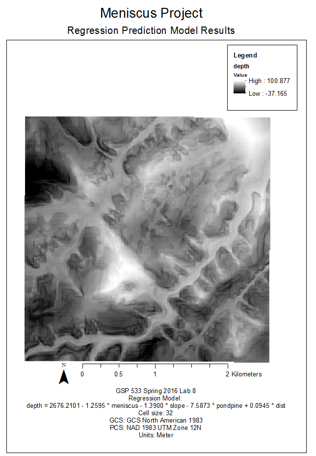
Finally, we input the resulting sample points feature class into the Ordinary Least Squares spatial regression tool using the Depth field as a parameter, and this operation created our soil depth prediction model equation.
This project has a lot of potential future work, especially when temporal aspects are considered. For example, the data analyzed was a snapshot of what's out there in the study area at time of data capture; private lands grow and shrink, stream channels change, changes in year-to-year rainfall can change the size of the canopy, etc.
Also, hydrologists studying their earthen dam's impact on the study area's watershed and indigent life depending on it could use the data we have collected and created.
The data gathering and manipulation processes of this project could be fully automated and running continously, again providing valuable information to decision makers showing how the project parameters of the study area are changing over time.
Finally, the ArcGIS software suite is not the only robust GIS suite out there. It is an expensive, proprietary, and highly protected piece of software; however, open source suites such as QGIS can in many cases provide as good or greater performance than ESRI's flagship product. Decision makers that know of the power of GIS software, but are mindful of the ArcGIS suite's cost, could instead utilize an open source alternative.
Primitive data types used by size:
Boolean, Integer (16-bit), Long Integer (32-bit), Character, String, Single precision floating point, Double precision floating point, Array, Object| Item | Type | Source | Projection | Filename | Date |
|---|---|---|---|---|---|
| uhh | uhh | uhh | uhh | uhh | uhh |